Visualizing Orientation in E3

I'm working toward a little laboratory for rigid-body simulation. For that, we need some more-or-less generic rigid bodies and a way of visualizing their positions and orientations in Euclidean 3-space (E3). E3 is good for now; we might get to curved spacetime later.

To get started, let's use Mathematica. Right out of the box, investigating 3D plotting from the help file, do this:

rcoord := {Random[], Random[], Random[]}
blarg[f_] := Module[{loc = f rcoord, siz = rcoord},
    Cuboid[loc,
      Table[loc[[i]] + siz[[i]], {i, 3}]]]
Show[Graphics3D[Table[blarg[3], {20}]], FaceGrids -> All, 

Axes -> True, AxesLabel -> {"x", "y", "z"},
    ViewPoint -> {1.3, -2.4, 2.}];

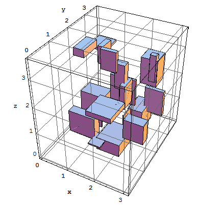Great. We have a way of spraying cubes around E3, and we can see their positions. Now, we need a way to track their orientations. The help file says "RotateShape" is the way to go. I found out by experimentation that "Cuboid" doesn't rotate like other graphics, so I made my own.

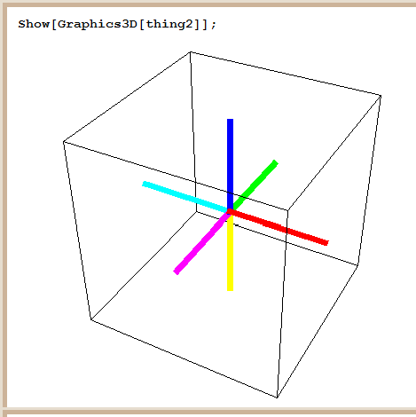
I wanted a color coding for the orientation of each of the six planes of a cube, so I came up with this. Let the unit vectors of the cube-fixed reference frame be x, y, z; in that order. Assign to their positive directions the primary colors, Red, Green, and Blue (RGB), in that order. Assign to their negative directions the complementary colors, Cyan, Magenta, and Yellow, respectively (CMY). The following illustrates:

thing2 = {Thickness[.02]
      , RGBColor[1, 0, 0]
      , Line[{{0, 0, 0}, {1, 0, 0}}]
      , RGBColor[0, 1, 0]
      , Line[{{0, 0, 0}, {0, 1, 0}}]
      , RGBColor[0, 0, 1]
      , Line[{{0, 0, 0}, {0, 0, 1}}]
      , RGBColor[0, 1, 1]
      , Line[{{0, 0, 0}, {-1, 0, 0}}]
      , RGBColor[1, 0, 1]
      , Line[{{0, 0, 0}, {0, -1, 0}}]
      , RGBColor[1, 1, 0]
      , Line[{{0, 0, 0}, {0, 0, -1}}]
      };

Embrace the right-hand rule and the wedge product for 2-forms, that is, for oriented planes, defining positive orientation for planes. Because of the lucky accidents that in E3 there are three basis vectors AND three planes, x^y, y^z, and z^x, plus three primary colors AND three secondary colors, we can unify color coding for vectors and planes:

x ~ y^z ~ Red   ~ {1,0,0},  -x ~ z^y ~ Cyan    ~ {0,1,1}
y ~ z^x ~ Green ~ {0,1,0},  -y ~ x^z ~ Magenta ~ {1,0,1}
z ~ x^y ~ Blue  ~ {0,0,1},  -z ~ y^x ~ Yellow  ~ {1,1,0}

Just to nail this down, hold up your right hand, thumb toward your face, and imagine the wrist bones on your pinky side touching the origin of the y^z plane, so that the plane's y basis vector points to the right and the plane's z basis vector points upward.

Let your fingers curl or sweep from the y direction to the z direction. Then, your thumb represents the x direction. If your thumb points at your face, then you should see Red, and if your thumb points away from your face, then you should see Cyan. That little procedure accounts for the first line above. Repeat for the other two lines, then convince yourself that you understand the following pictures. Their construction is a little too lengthy to reproduce in a blog entry.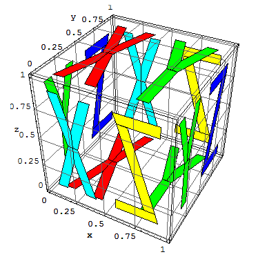

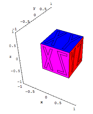
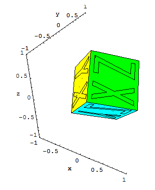
The final image below shows the body rotated with respect to the "world frame" and sets the stage for visualizing Newtonian rigid-body dynamical simulation. Again, make sure you can visually "parse" this image. The Green plane represents the body-fixed positive y ~ z^x axis and plane pointing at you. The Cyan plane represents the body-fixed negative x ~ y^z axis-plane pointing at you, or the positive ones pointing away from you. The Yellow plane represents the body-fixed positive z ~ x^y axis-plane pointing away from you, or, likewise, the negative ones pointing toward you.