Tumbling Video (experiment)

My friend Van of Warren Design Visions told me to post my tumbling video on youtube. Let's hope this works. If the embedded video doesn't show up, try

http://www.youtube.com/watch?v=Zne5cVXzPtA

A Famous Instability

Take a hardcover book that you don't mind dropping on the floor and put a couple of rubber bands around it to keep it closed. Observe that there are three axes of symmetry of the book: longest, shortest, and intermediate. Toss the book in the air so that it spins about the shortest axis. That's the axis that passes from the front of the book to the back (unless you have picked a very strangely shaped book). Try to catch it, too, but notice that the book starts off spinning around this axis, and continues spinning around this axis. This is a stable spinning motion. Now toss the book in the air so that it spins around the longest axis, most probably the axis from the top of the book to the bottom. Stable. Now, one more time, spin about the middle axis. Whoops! It won't stay spinning about that axis, but tumbles all over the place. UNSTABLE about the middle axis.

Somewhere in my vast library I have a theorem about this, which I'll try to resurrect for another blog. But this time I just want to point out that I've reproduced this behavior in my little Mathematica laboratory of rigid-body motion. I'm not sure how to publish a Flash movie on this blog, or, in fact, anywhere else on the web, but I do have one. Here's a snapshot:

I've got three versions of this movie, one showing stable spinning about the x (red) axis, another showing stable spinning about the y (green) axis, and the third showing UNstable spinning about the z (blue) axis. All three of them use the same 4th-order Runge-Kutta integrator of the rigid-body equations of motion for free spinning, which I coded up by hand in Mathematica. I'll be explaining this in future installments.

Fun with Shapes

rcoord:={Random[],Random[],Random[]}

eloof[f_]:=TranslateShape[
rotw[(2rcoord-1)Pi,AffineShape[wcube,rcoord]]
, f rcoord];

Depicting Rotations via Euler Angles

Here are the promised OBJECT-rotation operators. This actually took me much longer to explain than to create.

Using Mathematica once again, Consider a vector w representing angular velocity by its direction and magnitude. The direction specifies the axis of rotation and the magnitude specifies a positive twist rate in radians per unit time about this axis via the right-hand rule: thumb pointing along the axis, fingers curling in the sense of positive twist. To animate rotations, multiply w by dt to get dw, a small but finite actual rotation. Use "RotateShape," which documentation says "takes Euler angles," to depict such rotations.

Given dw's components, then, what arguments to supply to "RotateShape?" There are lots of different Euler-angle sets. This one turns out to be zxz frame-wise:

xaxis=Line[{{0,0,0},{1,0,0}}];
yaxis=Line[{{0,0,0},{0,1,0}}];
zaxis=Line[{{0,0,0},{0,0,1}}];

Look at the x axis after rotating about +z counterclockwise by a small angle, say p/6. If RotateShape rotates the FRAME, expect a small negative y contribution. If RotateShape rotates the OBJECT, expect a small positive y contribution:


Look at the y axis after a rotation about +x by a small angle. Expect small negative z contribution:

Picture an all-positive w, in the first octant of E3. To rotate the image of an object about such a w via "RotateShape," first get the frame's y axis directly under w by a negative twist about z, then do a negative twist about new x to get z aligned with w, then twist by negative mag[w], to twist the OBJECT rather than the frame, then undo the first two twists.

phi[w] is the angle w makes with the y axis, measured CLOCKwise from y to w in the xy plane. The first Euler angle should be a negative z twist by this angle.

theta[w] is the angle w makes with the z axis, measured counterclockwise from z to w in their common plane. The second Euler angle should be a negative x twist to align the new z axis with w.

Here's the rotation op:

And an animator for it:

And some evidence that it's working right

where

s3p=Show[Graphics3D[#
,FaceGrids->All
,Axes->True
,AxesLabel->{"x","y","z"}
,Lighting->False]
,ImageSize->Automatic]&;

This is good enough to support animation of rigid bodies in motion.

Models for Orientation Gadgets

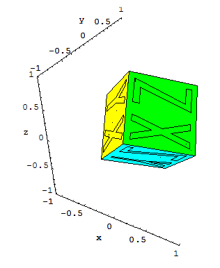
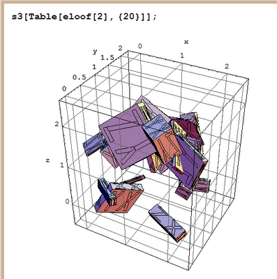
Here is some Mathematica code, without explanation, for improved orientation-visualization gadgetry. I'll do the display operators later, but I'm rushing out the door:

vcube=
TranslateShape[
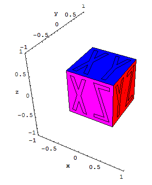
{FaceForm[RGBColor[0,0,1],RGBColor[1,1,0]]
,Polygon[{{0,0,0},{1,0,0}(*xy*)
,{1,1,0},{0,1,0}}]
,Polygon[{{0,0,1},{1,0,1}
,{1,1,1},{0,1,1}}]
,FaceForm[RGBColor[0,1,0],RGBColor[1,0,1]]
,Polygon[Reverse[{{0,1,0},{1,1,0}
,{1,1,1},{0,1,1}}]](*zx*)
,Polygon[Reverse[{{0,0,0},{1,0,0}
,{1,0,1},{0,0,1}}]]
,FaceForm[RGBColor[1,0,0],RGBColor[0,1,1]]
,Polygon[{{0,0,0},{0,1,0}
,{0,1,1},{0,0,1}}]
,Polygon[{{1,0,0},{1,1,0},{1,1,1}
,{1,0,1}}]
},{-.5,-.5,-.5}];

x2pols={FaceForm[RGBColor[0,0,0],RGBColor[.5,.5,.5]]
,Polygon[
Reverse[{{1,1,0},{2.5,6,0},{3,6,0},{3,4+1/3,0},{2,1,0}}/12.]]
,Polygon[
Reverse[{{4,1,0},{3,4+1/3,0},{3,6,0},{3.5,6,0},{5,1,0}}/12.]]
,Polygon[
Reverse[{{3,6,0},{2.5,6,0},{1,11,0},{2,11,0},{3,7+2/3,0}}/12.]]
,Polygon[
Reverse[{{3,6,0},{3,7+2/3,0},{4,11,0},{5,11,0},{3.5,6,0}}/12.]]
};

y2pols={FaceForm[RGBColor[0,0,0],RGBColor[.5,.5,.5]]
,Polygon[
Reverse[{{2.5,1,0},{2.5,6,0},{3.5,6,0},{3.5,1,0}}/12.]]
,Polygon[
Reverse[{{3,6,0},{2.5,6,0},{1,11,0},{2,11,0},{3,7+2/3,0}}/12.]]
,Polygon[
Reverse[{{3,6,0},{3,7+2/3,0},{4,11,0},{5,11,0},{3.5,6,0}}/12.]]
};

z2pols={FaceForm[RGBColor[0,0,0],RGBColor[.5,.5,.5]]
,Polygon[
Reverse[{{1,1,0},{1.3,2,0},{5,2,0},{5,1,0}}/12.]]
,Polygon[
Reverse[{{1.3,2,0},{3.7,10,0},{4.7,10,0},{2.3,2,0}}/12.]]
,Polygon[
Reverse[{{1,11,0},{5,11,0},{4.7,10,0},{1,10,0}}/12.]]
};

combp=Join[#1,TranslateShape[#2,{.5,0,0}]]&;

xy2p=combp[x2pols,y2pols];
yz2p=combp[y2pols,z2pols];
zx2p=combp[z2pols,x2pols];

face2labels=
TranslateShape[
{TranslateShape[RotateShape[zx2p,Pi,Pi/2,0], {1,0,0}]
,TranslateShape[RotateShape[zx2p,Pi,Pi/2,0],{1,1,0}]
,RotateShape[yz2p,0,-Pi/2,-Pi/2]
,TranslateShape[RotateShape[yz2p,0,-Pi/2,-Pi/2],{1,0,0}]
,xy2p
,TranslateShape[xy2p,{0,0,1}]},{-.5,-.5,-.5}];

wcube=Chop[Join[AffineShape[vcube,{0.99,0.99,0.99}],face2labels]];

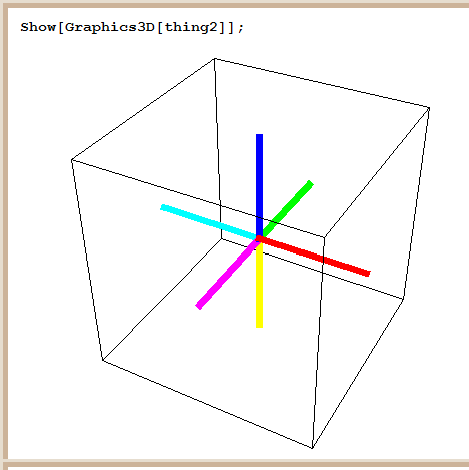
thing3={Thickness[0.010]
,RGBColor[1,0,0]
,Line[{{0,0,0},{1,0,0}}]
,RGBColor[0,1,0]
,Line[{{0,0,0},{0,1,0}}]
,RGBColor[0,0,1]
,Line[{{0,0,0},{0,0,1}}]
,RGBColor[0,1,1]
,Line[{{0,0,0},{-1,0,0}}]
,RGBColor[1,0,1]
,Line[{{0,0,0},{0,-1,0}}]
,RGBColor[1,1,0]
,Line[{{0,0,0},{0,0,-1}}]
};

xcube=Join[AffineShape[thing3,{2,2,2}],wcube];

Visualizing Orientation in E3

I'm working toward a little laboratory for rigid-body simulation. For that, we need some more-or-less generic rigid bodies and a way of visualizing their positions and orientations in Euclidean 3-space (E3). E3 is good for now; we might get to curved spacetime later.

To get started, let's use Mathematica. Right out of the box, investigating 3D plotting from the help file, do this:

rcoord := {Random[], Random[], Random[]}
blarg[f_] := Module[{loc = f rcoord, siz = rcoord},
    Cuboid[loc,
      Table[loc[[i]] + siz[[i]], {i, 3}]]]
Show[Graphics3D[Table[blarg[3], {20}]], FaceGrids -> All, 

Axes -> True, AxesLabel -> {"x", "y", "z"},
    ViewPoint -> {1.3, -2.4, 2.}];

Great. We have a way of spraying cubes around E3, and we can see their positions. Now, we need a way to track their orientations. The help file says "RotateShape" is the way to go. I found out by experimentation that "Cuboid" doesn't rotate like other graphics, so I made my own.

I wanted a color coding for the orientation of each of the six planes of a cube, so I came up with this. Let the unit vectors of the cube-fixed reference frame be x, y, z; in that order. Assign to their positive directions the primary colors, Red, Green, and Blue (RGB), in that order. Assign to their negative directions the complementary colors, Cyan, Magenta, and Yellow, respectively (CMY). The following illustrates:

thing2 = {Thickness[.02]
      , RGBColor[1, 0, 0]
      , Line[{{0, 0, 0}, {1, 0, 0}}]
      , RGBColor[0, 1, 0]
      , Line[{{0, 0, 0}, {0, 1, 0}}]
      , RGBColor[0, 0, 1]
      , Line[{{0, 0, 0}, {0, 0, 1}}]
      , RGBColor[0, 1, 1]
      , Line[{{0, 0, 0}, {-1, 0, 0}}]
      , RGBColor[1, 0, 1]
      , Line[{{0, 0, 0}, {0, -1, 0}}]
      , RGBColor[1, 1, 0]
      , Line[{{0, 0, 0}, {0, 0, -1}}]
      };

Embrace the right-hand rule and the wedge product for 2-forms, that is, for oriented planes, defining positive orientation for planes. Because of the lucky accidents that in E3 there are three basis vectors AND three planes, x^y, y^z, and z^x, plus three primary colors AND three secondary colors, we can unify color coding for vectors and planes:

x ~ y^z ~ Red   ~ {1,0,0},  -x ~ z^y ~ Cyan    ~ {0,1,1}
y ~ z^x ~ Green ~ {0,1,0},  -y ~ x^z ~ Magenta ~ {1,0,1}
z ~ x^y ~ Blue  ~ {0,0,1},  -z ~ y^x ~ Yellow  ~ {1,1,0}

Just to nail this down, hold up your right hand, thumb toward your face, and imagine the wrist bones on your pinky side touching the origin of the y^z plane, so that the plane's y basis vector points to the right and the plane's z basis vector points upward.

Let your fingers curl or sweep from the y direction to the z direction. Then, your thumb represents the x direction. If your thumb points at your face, then you should see Red, and if your thumb points away from your face, then you should see Cyan. That little procedure accounts for the first line above. Repeat for the other two lines, then convince yourself that you understand the following pictures. Their construction is a little too lengthy to reproduce in a blog entry.

The final image below shows the body rotated with respect to the "world frame" and sets the stage for visualizing Newtonian rigid-body dynamical simulation. Again, make sure you can visually "parse" this image. The Green plane represents the body-fixed positive y ~ z^x axis and plane pointing at you. The Cyan plane represents the body-fixed negative x ~ y^z axis-plane pointing at you, or the positive ones pointing away from you. The Yellow plane represents the body-fixed positive z ~ x^y axis-plane pointing away from you, or, likewise, the negative ones pointing toward you.

Euclid Tougher than Minkowski

We've done a few Geometry Expressions demos showing off Minkowski geometry and how it solves problems in Special Relativity. How about Euclidean geometry? The usual 2D rotation diagram is easy enough to set up. Let point B have coordinates x,y. Let the red frame be rotated by angle theta with respect to the blue frame and ask "What are the coordinates of B in the red frame?" We all remember the answer: x' = x cos theta + y sin theta, y' = - x sin theta + y cos theta. What does GX say?


JF is obviously (BD = x) cos theta, as is IC = (AC = x) cos theta, just by looking at the picture. Ditto HF = (BC = y) sin theta, and the y' coordinate is just as easy to see. Mathematica's simplification machinery is better than GX's, and it's a simple matter to copy-as and paste back to Mathematica,


I'm getting quite accustomed to this procedure. It's amusing as well as useful.

GX file for you to download is at http://home.comcast.net/~brianbec/Euclidean3.gx

Velocity Addition for Free

Ever go through the traditional derivation of the relativistic formula for addition of velocities? Painful, because there are a bunch of things you have to hold in your head for the duration of a calculation. Modern tools make this easy, almost obvious. First, recall this sketch:

in which Geometry Expressions calculates the Lorentz transformation for free. Now, suppose the point B really represents the endpoint of a particle path, the beginning-point being the origin (0,0). In the blue frame -- our lab frame -- the (average) velocity of the particle over this path is x/t, which we can write as u. What's the velocity of the same particle path, this time measured in the red frame, moving with velocity v w.r.t. our blue frame? Why, let's let Mathematica compute it for us. Use the "Edit / Copy As / Mathematica" menu item in Geometry Expressions on the yellow expressions in the sketch above, and just paste into Mathematica:

Beautiful simplicity itself, eh? Once again, I've been lazy with absolute-value expressions, just sidestepping them. This means the signs -- but only the signs -- may turn out wrong and we would have to use common sense to correct them.

Double Doppler for Free

The last post showed the relativistic Doppler effect measured in a stationary frame from bouncing signals off an object in a moving frame. How about two moving frames? Geometry Expressions does a really good job, but, this time, the results are sufficiently hairy that we must help out a bit. The Minkowski sketch is simple enough -- one frame has speed u and the other has speed v.

I chopped off this very hairy expression for the pulse duration in the v frame:

We all know that simplifying algebraic expressions is a tough problem, and sometimes doesn't give the results we want. So, I used GX's "copy to Mathematica form", and, after a FullSimplify in MMA, got this:

This still wasn't good enough for me, so, by hand, I figured this:

But, symbolic checking of equality is problematic because of the absolute-value functions, resulting from the fact that we didn't constrain u and v adequately to be less than one = c. I'm lazy, so I checked equality numerically:

More Minkowski for Free

Here's a nice relativistic analysis of an experiment, building on the framework in the last blog (at http://weblogs.asp.net/brianbec), calculations courtesy of Geometry Expressions once again. Think of laser ranging to the moon. The astronauts left mirrors on the moon, and every day pulses are shot at the mirrors, which are actually corner reflectors, so the pulses bounce straight back. The moon is about 1.5 light-seconds away, so the round trips take about 3 seconds. The moon is moving about 2300 miles per hour, which is about 3e-6 times the speed of light, so the pulses are lengthened by (at most) microseconds, which is very easy to measure with modern equipment, so relativity is spectacularly verified every day in experiments like this.

As before, the blue axes are our non-moving lab frame, and the red axes are a frame of reference moving at velocity v in the x direction. The pulse begins at event A and ends at event J in our blue frame. The red (moon) frame sees the pulse beginning at event Q and ending at event B. The line CB is a line of constant position -- say, the position of the mirror -- in the red moon frame. When we get the pulse back on Earth, it has been stretch to duration RK. This is relativistic Doppler shifting of light.

Here's a slightly prettier picture.

The files are http://home.comcast.net/~brianbec/Minkowski.gx and http://home.comcast.net/~brianbec/Minkowski3.gx